With the accelerometer project completed, the natural place to test it was on various amusement rides at DisneyWorld in Florida. Presented are the data recorded on several rides including Tower of Terror (my favourite), Mission Space, and Rockin Roller Coaster. Tower of Terror is my favourite analysis – it is one axis only so simple physics can be used to determine velocity and position.
The Basic Physics
 An accelerometer measures “proper acceleration”, which is the physical acceleration an object experiences resulting from either motion or from gravity. We often say that an accelerometer measures “g-force” but this is actually not a force at all – rather what is felt is the force of the earth pushing upwards on the observer preventing them from entering a free fall. Consider Mickey in an elevator (as depicted on the left). While Mickey might “feel” the “pull” of gravity, the real force is exerted upwards by the elevator. A stationary accelerometer will hence read “+1g”.
Now, in a free-fall gravity acts on a mass to accelerate it towards the earth. Since nothing pushes upwards on the observer (here, Mickey) feels weightless. The scale upon which Mickey is standing would read zero and an accelerometer in the elevator would read also zero.
So, we often speak of gravity as a “force” but it is really an acceleration – what we feel as gravity is the force that the earth exerts upwards to keep object from entering a free-fall. Regardless of definition, acceleration is often measured in units of “g’s” with one “g” defined as an acceleration of 9.8 m/s2.
A similar situation exists in an accelerating vehicle in which the user feels pushed back into the seat. The actual force is in the forward direction and is, in fact, the force of the vehicle pushing on the passenger.
Raw Data
The accelerometer, which uses an Analog Devices ADXL312 accelerometer chip, records acceleration in three axes in the range +/- 12g as signed numbers with 12-bits of resolution. Sitting on a desk, for example, the Z-axis will read, numerically, about 345 (the resolution of the device, then, being about 2.9 milli-G’s). In reality, the accelerometer in this device is mounted upside-down due to the necessity to attach leads to the package in which it is supplied (this is then inverted in a spreadsheet although the newer firmware revision does this inside the device.
To record a run, the user simply selects the RECord function and data is stored into a large internal flash memory chip. Data from the chip can then be downloaded serially. The resulting data is in CSV (Comma Separated Value) format with the first number a sequence number, and the resulting three numbers the acceleration values per the following example:
04406,00013,-00582,-00029
04407,00016,-00563,-00017
04408,00021,-00559,-00026
04409,00009,-00561,-00003
04410,00003,-00545,-00012
04411,00011,-00537,-00002
04412,00009,-00528,-00010
04413,00011,-00509,-00028
04414,00009,-00473,-00013
04415,00015,-00447,-00010
In this example, the unit was oriented such that the Y axis is in the vertical (up/down) direction and so the X (column two) and Z (column four) readings hover around zero as expected. There are not many flat surfaces in a ride to mount this device (nor time to look around) so the device was attached to the first steel post found. Inversion of the axis (so that, for example, it reads “+1g” when stationary and not “-1g”) is accomplished in the spreadsheet quite easily.
There is a small offset error from the device itself which could have been eliminated by using the self-calibration feature of the ADXL chip (but was not used in this case so small errors must be corrected during analysis). The third column shows an acceleration of approximately -560 or -1.6g but since the unit is actually inverted, the real force is +1.6g (the upwards force of the elevator on the passengers as it rises rapidly. You’ll notice as well that all three columns show a noise figure in which the signal varies randomly even with the device sitting still – some of this noise is generated by the shaking of the ride vehicle and some is electrical in nature.
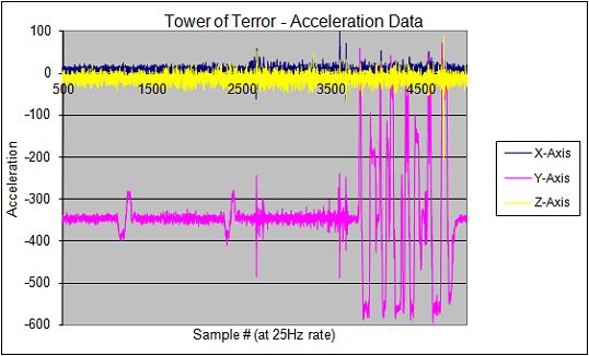
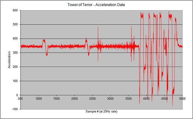
After loading into the ride vehicle, the car ascends at around sample 1200 (the first bump on the graph) – the ride car accelerates upwards, then decelerates to a stop. After a short pause the car accelerates again (around 2400, or about 48 seconds later). The ride car loads into the main drop shaft (the two noisy bumps between 2500 and 3500), and the drops occur. In this case, the ride car encounters a drop on the first entry to the shaft (the first large spike after 3500) resulting in a weightless condition of 0g (actually, the ride car accelerates downward faster than gravity – you literally float out of your seat as the ride car is pulled out from under you!).
Analysis
The device provides only acceleration data (in units of g’s or, converted, m/s2). Velocity may be found by integrating acceleration with respect to time. Integrating velocity will then result in position.
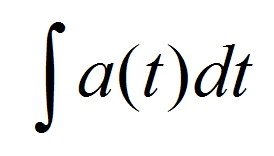 Now, if the acceleration could be determined as a function of time, i.e. the function a(t) could be developed from the observed data, determining velocity would be a simple matter of integrating acceleration with respect to time. If, for example, acceleration was constant the solution to the integral is simply v=at+k where k is a constant (it will solve to the initial velocity of the object before the acceleration occurred, namely v0). Unfortunately, real-world object rarely accelerate at a constant rate as is clear from observing the acceleration data recorded, and so a numerical approach is warranted here.
The numerical approach is not magic, it is simply that of using a finite time interval Δt (instead on the infinitely small dt used with an integral) and, assuming that the interval chosen is very small, acceleration is essentially constant during that interval. It isn’t absolutely constant, of course, but if the change of acceleration is small between samples the answer is valid and has a relatively small error from the expected “proper” solution found using calculus.
In the specific case of this data, a simple numerical method may be used to determine velocity by multiplying acceleration times Δx (which is 40ms in this case where a 25Hz sample rate is employed). A spreadsheet was used to analyze this data as follows:
- The nominal value for one-g is found by averaging several hundred samples while the ride car is stationary. In theory, any one value would work but due to noise in the system, an average is taken. This value is, numerically, approximately 345.
- Raw acceleration data is converted into acceleration in units on m/s2 by dividing the value from the accelerometer by the nominal value for one g (above) and multiplying by 9.8m/s2. This represents the instantaneous acceleration at this time, i.e. a(t) during the time interval Δt.
- Instantaneous change in velocity (during the interval Δt) is found by multiplying acceleration by Δt (40ms for the sample rate of 25Hz employed) then adding the last known value for velocity (in other words, integrating the velocity, in which case the “last known value” for velocity is v0 and is that found during the previous time interval). The basic equation is v(t) = v(t-1)+a(t)*Δt since a(t)*Δt represents the change in velocity during the time Δt and v(t-1) the velocity determined during the last time interval. In the spreadsheet this is found by adding the value for velocity in the previous row to the value of acceleration (above) times 0.040. This is in units of m/s.
- Position is found by multiplying velocity by Δx and summing with the previous value of position (again, integrating it). If you look at it that way, x(t) = x(t-1)+v(t)*Δt. This may also be interpreted as the ‘traditional’ physics kinematics formula x(t) = x0+1/2*a*Δt2 where x0 is the position from the last time period. This formula is used in physics where acceleration is constant over a known time period – in our case the time period is very small (the smaller, the more accurate the simulation).
Spreadsheets are wonderful tools for data analysis such as this and lend themselves well to numerical methods. Having employed them for analysis of laser systems I use them here to calculate the motion of the ride car. Data was downloaded to a spreadsheet and several calculations added in adjoining columns as seen here:
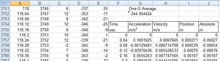
Implementation of the spreadsheet is perhaps best illustrated by example. Consider row 3757 which has the following formulae:
F3757=F3756+(1/25) //Calculates the time elapsed from zero (which is defined arbitrarily, in this case as the point where the lift sequence begins
G3757=((1-1*D3757/$G$3752)*9.8) //Calculates net acceleration (subtracting 1g for gravity) and then converting to units of metres per second-squared. Cell $G$3752 is an average “zero” value for +1g.
H3757=H3756+G3757*(1/25) //Calculates velocity as a function of initial velocity (from the last row), and current acceleration
I3757=I3756+H3757*(1/25) //Calculates position as a function of initial position (from the last row), and current velocity
J3757=-1*I3757 //Calculates absolute position from the starting point, correcting for the orientation of the device
formulae from this row are now simply copied to the next 2500 rows causing row references to increment each time (so “F3756” increments on the next row to “F3757” and so on).
Position data may then be graphed (Time in column “F” on the x-axis, and Position in column “J” on the y-axis). With two integrations, it is easy to see how even a small error can result in large errors at the end so each drop sequence was treated separately to avoid cumulative error (seen as “drift” in plots where the ride car remains stationary but the graph continues to slowly climb or fall). The first part of the ride analyzed was the ascent which occurs after guests are loaded into the ride car:
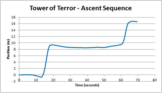
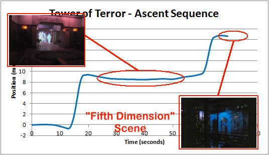
Clearly visible here are two lift sequences. The first brings riders from the loading level (in reality, the second floor of the ride) to a middle position where a twilight-zone-esque video sequence is played. A second lift brings riders to approximately the fifth floor where the ride car travels to the main drop shafts. The data shows, as expected, the load to the main drop shaft occurs at a level of 17m above the loading level (already the second floor).
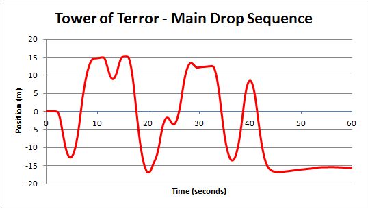
The main drop sequences are always random on this ride. In this case the first drop occurs immediately after loading into the main shaft. Following that, a sequence of drops, including one large drop, occurs over the next 45 seconds. Finally, the car comes to rest – the graph shows this position to be about 17m below the start position but in reality is would be about one floor lower where guests are unloaded. “Zero” is taken to be the loading position however for absolute position, it should be set to 17m (from the ascent, described previously)
Those who have rode the Tower of Terror will recognize several drop sequences such as the small drop at the top of the shaft (around 12 seconds) in which the car flies to the top of the shaft (allowing guests to see over the entire park), makes a small drop, returning to the top (a “teaser” if you will), followed by a massive drop which pulls you upwards from the seat (the car is actually pulled downward by the ride motors and so is falling faster than a free-fall at that point – verified from the acceleration data). Another feature is the second rise to “almost” the top of the shaft (just below the doors at the top), again with a slight drop and rise, followed by a large drop.
The full data set, along with complete analysis, can be found in this file: DisneyTowerOfTerror. This is an XLS spreadsheet from Excel 2007. The Y-axis is corrected for polarity (the fact that the accelerometer is inverted) and graphs are embedded into the spreadsheet.
Validity Of This Approach
As stated earlier, the numerical approach is valid only if the acceleration change between samples is small. By simple observation of the data from this ride it can be found that during the largest drop sequence the change in acceleration between two adjacent samples (i.e. over the time period Δt=40ms) averages only 0.12g’s when the data is filtered (using a simple sliding window algorithm) to reduce noise. This is a relatively small value considering it is 7% of the maximum value of acceleration recorded and so logically one expects a final error of under 10% … indeed data recorded on the Rock ‘n Roller Coaster (below) seems to indicate a 10% discrepancy between recorded and accepted values.
Use of a higher sample rate (which the ADXL chip will already support) and a better filtering algorithm to suppress random noise will both help the accuracy of this device.
Rock’n Roller Coaster Analysis
 One of the fastest rides at DisneyWorld in Florida, Rock ‘n Roller Coaster is a steel roller coaster completely enclosed in a building. It features a unique electromagnetic launch system (a linear motor, really) which propels the car from zero to sixty MPH in 2.8 seconds!
Like most roller coasters, analysis is difficult with acceleration data alone, however the launch system is quite interesting to analyze. First issue: there is no ferrous metal on the ride so the accelerometer was held-down by sitting on it. Since the seats in the ride car are at an angle, a bit of simple physics (in the form of vectors) is required to determine the actual acceleration.
Examining the data from the ride, it can be seen that just before launch (at time t=0) the X axis (front-back) is not zero as expected but shows a nominal value of 0.427G: determined by knowing (from data for the Tower of Terror above) that 1G produces a reading of 344.892. The average reading of the stationary X-axis is 147.5 or 0.427G. Similarly, the Z-axis should read 1G when stationary but reads 0.906G instead.
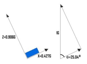 First, it can be noted that the X and Z accelerations are at right angles to each other so, using the Pythagorean theorem, we obtain a hypotenuse (the actual acceleration in the Z-axis) = √ 0.427 2+0.906 2 = 1.002G as expected.
Simple mathematics can now be used to determine that the accelerometer is inclined at an angle of 25.04 degrees and so, using simple trigonometry, the actual X-axis acceleration is:
The “correction factor” of 1/cos(25.04 degrees),or 1.104, simply means that the actual acceleration in the X-axis is the net acceleration (minus gravity) measured by the inclined accelerometer multiplied by 1.104.
This illustrates how to handle data from the unit even when it is not mounted optimally “flat” to an axis (as it was for the Tower of Terror analysis).
The velocity is then determined by numerically integrating the acceleration as per the same methodology as used with the Tower of Terror analysis. It was found that 2.8 seconds after the acceleration begins, the ride car reaches a velocity of 23.25 m/s (52mph). Errors in the recorded measurements are the likely cause of discrepancy between this and the “accepted” value of 57mph.
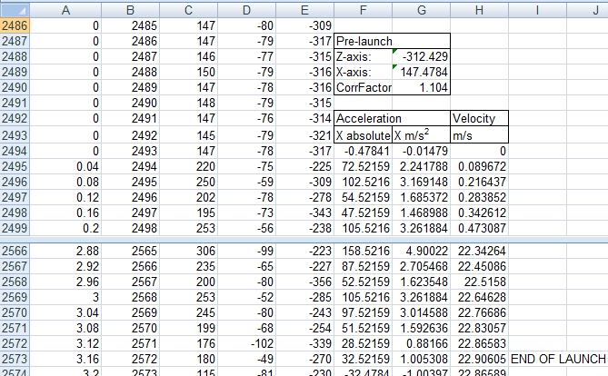
Launch data for Rock ‘n Roller Coaster. Time is seen here in column A (with “zero” re-defined as the start of the launch sequence where acceleration increases sharply) as well as “raw” accelerometer data in columns B, C, and D. Absolute acceleration (in column F) is computed by subtracting the “idle” offset in cell G2489 (an average of a large number os readings taken when the ride car was stationary just before launch). Acceleration is then converted into units of m/s2 in column G. Numerical integration is then done to convert to velocity in column H. Shown are the start of the launch (where velocity is defined as zero) and the end of the launch where velocity is 22.9m/s.
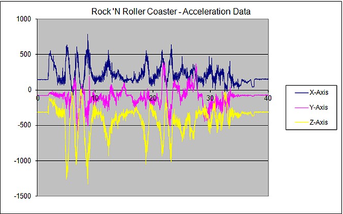
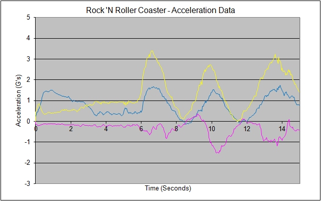 Processed data for the first fifteen seconds shows the launch sequence as well as the first loop which is actually a half-loop followed by an inversion and a second half-loop. The data seen here has zero defined when launch starts (as above) and is filtered using a moving-average algorithm with a window size of four to reduce noise. Acceleration data is converted into units of “G’s” and the Z-axis (yellow) is corrected for the upside-down sensor as noted in the beginning of this page. The half-loop is evident at six seconds as acceleration in the Z-axis rises sharply: when in the loop, the apparent reactive centripetal force is in the direction towards the outside of the loop (the real force is the track pushing against the car, or the car pushing against the rider who now feels as if he/she is being pushed into the seat).
Mission Space Analysis
Unlike the Tower of Terror, the accelerometer cannot be used to determine position – not that it’d be all that interesting, since the ride simply spins in a circle, however the accelerometer cannot sense rotation … for this a gyroscope is required. And so, the data is presented simple as acceleration data.
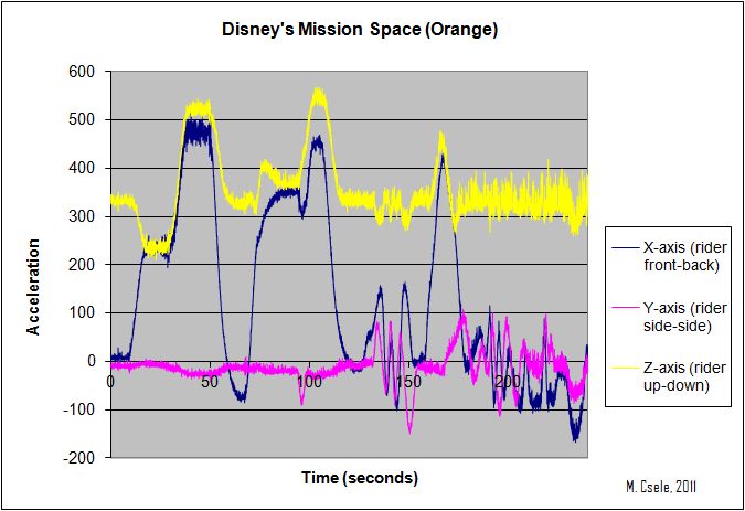
For the Mission Space ride, the accelerometer was attached to the ferrous metal underside of the console. When the console was pulled forward after loading, it was evident that the accelerometer was almost perfectly horizontal (since the X and Y axes both read zero and the Z axis reads 1.0g upwards). The accelerometer, at this point, is upside-down so that the Z-axis shows a force of +1g (i.e. upwards) not -1g (i.e. downwards) as expected (remember, the accelerometer chip was inverted in the device).
The ride begins at about 8 seconds where the seat reclines so that the rider is almost horizontal (as seen by the decrease in the Z-axis force and the corresponding increase in the X-axis force. The X-axis is now almost horizontal). The rider is left in this position for ten seconds during “launch countdown” after which the ride car is tilted in the axis of the spinning resulting in a large g-force in the X and Z axes. Although the force in each direction appears to be about 1.5 g’s, the RMS value (calculated by squaring the g-force in each value, summing these squares, and taking the square root) is very close to 2.0 (the “rated” g-force of this attraction). We then achieve “zero g”, simulated by having the X-axis force run from +1.5g to just below 0g by changing the axis of the ride vehicle, again, relative to the spinning axis … the feeling of going from a large downward force to a small force is perceived as “weightlessness” (and you certainly feel the force pushing you into the seat as being released so the effect is quite convincing). The second stage rocket is engaged at about 67 seconds and another large force is felt by the rider as we travel past the space station towards the moon, followed by “trans-lunar insertion”. Another “weightless” sensation during hypersleep is followed by a turbulent ride through asteroids (just before 150 seconds on the graph). Finally, a quick descent to the Martian surface (pulling a large g-force in the process) and a navigating over the mountainous terrain is followed by the “hanging over the cliff” motion at the end (where the X axis rotates so that the car is tipped forward – seen as the X axis going to about -0.3g).
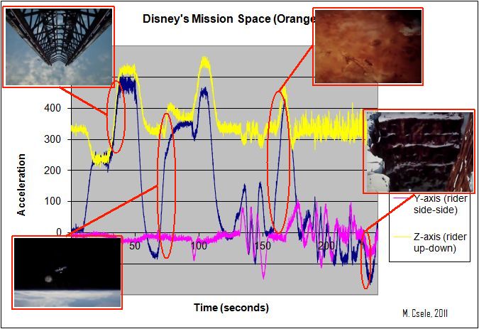
If you wish to correlate the acceleration data to the actual ride visuals, simply go to YouTube and search “Mission Space”. By examining the run time of the video and the acceleration data together, you’ll get an idea of how it all fits together! The above graph shows where a few scenes from the attraction fit.
This is, of course, the “updated” ride which is generally agreed to be more tame than the original version (which pulled more “g’s”). Still, at over 2g’s (sustained for over ten seconds), the rider does feel a significant force!
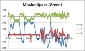 Acceleration from the “Green Team” ride (seen here as raw data, corrected for the fact that the unit was oriented differently than the orange team above) shows similar, but considerably smaller, forces. Since the “green” ride features no spinning, the simulator cars can move only in the Z and X axes and the g-forces are limited to the range -1g to +1g (and at that, -1g would require the rider to be upside-down which does not occur here). So the “weightless” simulation is simply a turn of the ride car from a horizontal position to vertical again.
Expedition Everest Analysis
This is the most “vicious” roller coaster at Walt Disney World, and riders are subject to serious g-forces both during the forward and backward portions of the ride.
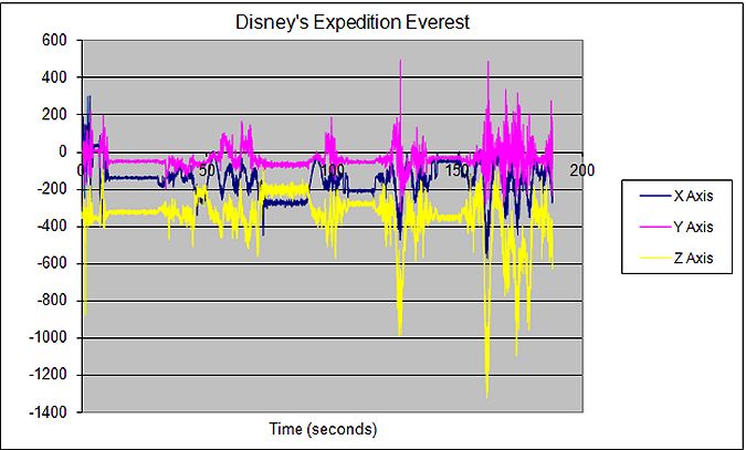
The ride begins at time t=30 seconds (after loading) where the ride car is released. Eight seconds later, after a gentle turn, the car is raised over a short hill and travels to the main lift which begins at 72 seconds as evident from the graph in which the Z-axis force is reduced and the X-axis force is increased indicating a tilt. The lift takes about 50 seconds to reach the top of the mountain, travels downward eventually reaching the “broken track” at 106 seconds. The track behind the car switches (taking about twelve seconds to do this), and travels backwards at high velocity around a sharp bend pulling a whopping FOUR RMS g’s (although this is a peak value recorded only for a transient moment – a figure of over 3 g’s was recorded for over two seconds during the backwards segment of the ride though). Later, during the forward segment of the ride (the large drop ending with a sharp turn at the bottom), a value of about 2.5 g’s (sustained for 1.5 seconds) is felt.